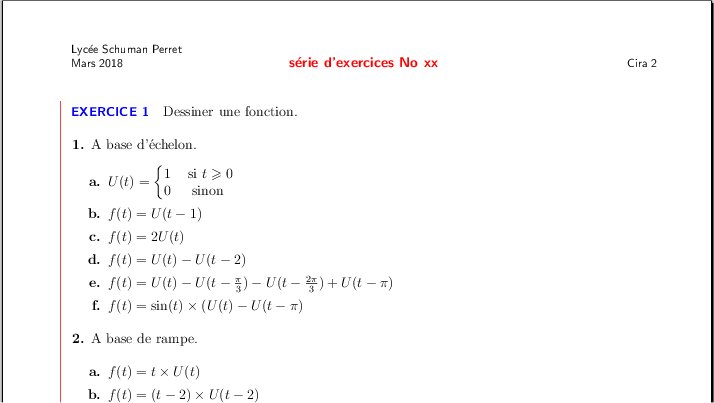
Qu est ce ?
$\LaTeX$ est un langage et un système de composition de documents créé par Leslie Lamport
écrit par : steph, le 30/07/2017 Lu par tous
Tableau de signes
Avec le package \usepackage{tikz,tkz-tab}
Pour gérer la largeur de la première colonne on peut jouer avec lgt
La documentation complète est là
Pour gérer la largeur de la première colonne on peut jouer avec lgt
\begin{tikzpicture}
   \tkzTabInit[lgt=3]{$x$ / 1 , $x^2-3x+2$ / 1}{$-\infty$, $1$, $2$, $+\infty$}
   \tkzTabLine{,+, z, -,z,+, }
\end{tikzpicture}
écrit par : steph, le 01/08/2017 Lu par tous
Arbre de probabilités
Je me suis battu en vain avec pstplus et finalement la documentation de pstree est largement suffisante.
\psset{treemode=R,nodesep=1mm,levelsep=20mm,treesep=5mm}
%\pstree[treemode=R,levelsep=15ex]{\Tcircle{R} }{
\pstree{\TR{$\Omega$} }{
\pstree{ \Tcircle{$A1$}\taput{$\frac18$} }
    {
    \pstree{ \Tcircle{$A2$}\taput{$\frac18$} }
        {
        \Tcircle{$A3$}\taput{$\frac18$}
        \Tcircle{$\overline{A3}$}\tbput{$\frac78$}
        }
    \pstree{ \Tcircle{$\overline{A2}$}\taput{$\frac78$} }
        {
        \Tcircle{$A3$}\taput{$\frac18$}
        \Tcircle{$\overline{A3}$}\tbput{$\frac78$}
        }
    }
\pstree{ \Tcircle{$\overline{A1}$}\taput{$\frac78$} }
    {
    \pstree{ \Tcircle{$A2$}\taput{$\frac18$} }
        {
        \Tcircle{$A3$}\taput{$\frac18$}
        \Tcircle{$\overline{A3}$}\tbput{$\frac78$}
        }
    \pstree{ \Tcircle{$\overline{A2}$}\taput{$\frac78$} }
        {
        \Tcircle{$A3$}\taput{$\frac18$}
        \Tcircle{$\overline{A3}$}\tbput{$\frac78$}
        }
    }
}
|

|
écrit par : steph, le 17/08/2017 Lu par tous
Arbre de probabilités (2)
\documentclass [a4paper,10pt] {article}
\usepackage [latin1]{inputenc}
\usepackage [T1]{fontenc}
\usepackage [francais]{babel}

\usepackage{amsmath,amsfonts,amssymb}
\usepackage{mathrsfs,eurosym}
\usepackage{pstricks,pst-plot,pst-eucl}
\usepackage{pst-tree}

\begin{document}

Un peu de baratin avant \bigskip

\begin{minipage}{0.4\linewidth}%une minipage pour le premier arbre
% Créé avec PST+ et modifié à la main
\psset{nodesep=1mm,levelsep=20mm,treesep=10mm}
\pstree[treemode=R]{\Tr{$\Omega$}}
{\pstree[ref=c]
   {\Tr{${\rm B}$}\naput{\small $\frac{1}{10}$}}
   {\Tr{${\rm G}$}\ncput*{\small $\frac{5}{6}$}
    \Tr{$\bar{\rm G}$}\nbput{\small $\frac{1}{6}$}}
 \pstree[ref=c]
   {\Tdot~[tnpos=b]{$\bar{\rm B}$}\tbput{\small $\frac{9}{10}$}}
   {\Tdot~[tnpos=a]{${\rm G}$}\taput{\small $\frac{1}{6}$}
    \Tdot~[tnpos=r]{$\bar{\rm G}$}\tbput{\small $\frac{5}{6}$}}
}
\end{minipage}\hfill

\bigskip Un peu de baratin après
\end{document}
|
|
écrit par : steph, le 18/08/2017 Lu par tous
Boites
Package fancybox
Package tcolorbox
Des boites de toutes les couleurs extrêmement paramétrables.
\fcolorbox {couleur de la police}{couleur du fond}{contenu)
\ovalbox{contenu}
Des boites de toutes les couleurs extrêmement paramétrables.
écrit par : steteil, le 28/09/2017 Lu par tous
Tableaux et tabulation automatique.
Créer un tableau avec des colonnes de taille fixe et centrées
\def\taille{\vrule height 20pt depth 20pt width 0pt }
    \begin{tabular}{*{4}{|>{\centering}p{3cm}}|}
    \hline
    \taille $a$ & $b$ & $c$ & $d$\cr
    \hline
    \end{tabular}
Le package spreadtab permet d'utiliser un tableur basique, il est pratique pour tabuler automatiquement des fonctions, des suites, etc.
\begin{spreadtab}{{tabular}{|c|*{13}{c|}}}
 \hline
 @$x$ & 0 & \STcopy{>}{b1+0.5} & & & & & & & & &&&\\\hline
 @$f(x)$ & \STcopy{>}{-0.08*b1*b1+0.8*b1+1.92} & & & & & & & & &&&&\\\hline
\end{spreadtab}
écrit par : steteil, le 03/10/2017 Lu par tous
Variations
Les beaux tableaux sont décrits ici :
http://distrib-coffee.ipsl.jussieu.fr/pub/mirrors/ctan/macros/latex/contrib/tkz/tkz-tab/doc/tkz-tab-screen.pdf
\usepackage{tikz,tkz-tab}

\begin{tikzpicture}
\tkzTabInit{$x$/1,$1-x$/1,$f'(x)$/1,$f(x)$/2}{$0$,$1$,$+\infty$}
\tkzTabLine{ ,+,z,-}
\tkzTabLine{ ,+,z,-}
\tkzTabVar{-/$0$,+/$f(1)$,-/$0$}
\end{tikzpicture}
écrit par : steteil, le 10/10/2017 Lu par tous
Enumerate
Ceci permet de réduire l'intentation de second niveau
\usepackage{enumerate}

\begin{enumerate}
\item machin
    \begin{enumerate}[\hspace{-30pt}a)]
    \item  truc
    \end{enumerate}
\end{enumerate}
écrit par : steteil, le 14/01/2018 Lu par tous
Boucle
Avec le package Tikz, on dispose de la possibilité de boucle.
Il suffit de déclarer le compteur dans le préambule avec un
Il suffit de déclarer le compteur dans le préambule avec un
\newcounter{mt}
puis on l'utilise, ici dans une fonction :
\def\anti#1{\loop\stepcounter{mt}\!\ifnum\value{mt}<#1\repeat}
Cette boucle permet de règler les espaces négatifs dans une intégrale, lorsque la fonction est trop loin du signe somme à mon gout.
écrit par : steph, le 09/02/2018 Lu par tous
Réduire l'indentation des listes
\usepackage{enumerate}

\begin{enumerate}
\item machin
    \begin{enumerate}[\hspace{-30pt}a)]
    \item  truc
    \end{enumerate}
\end{enumerate}
ou avec
\usepackage{paralist}

\setdefaultleftmargin{0.6cm}{0.5cm}{}{}{}{}
écrit par : steteil, le 09/02/2018 Lu par tous
Lignes et boites
- une ligne pour séparer des parties : RULE
\hfil\rule{8cm}{0.2mm} - aligner des minipages en haut: [t]
\begin{minipage}[t]{0.55\linewidth}
écrit par : steteil, le 09/02/2018 Lu par tous
Simuler un tableur
\usepackage{pas-tableur}\usetikzlibrary{math}
Puis :
\begin{tikzpicture}[thick,scale=0.6, every node/.style={scale=0.6}]
\tableur[12]{A-B}
\celtxt[c]{A}{1}{Valeurs}
    \foreach \x in {2,...,10}
    {
    \pgfmathtruncatemacro\z{7*\x+1-\x*\x/5};
    \celtxt[c]{A}{\x}{\z}
    }
\selecCell {A}{11}
\end{tikzpicture}
ou bien
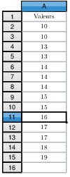
\begin{tikzpicture}[thick,scale=0.6, every node/.style={scale=0.6}]
\tikzmath{
\x1 = 10;
\x2 = 10;
\x3 = 13;
\x4 = 13;
\x5 = 14;
\x6 = 14;
\x7 = 14;
\x8 = 15;
\x9 = 15;
\x{10} = 16;
\x{11} = 17;
\x{12} = 17;
\x{13} = 18;
\x{14} = 19;
}
\tableur[16]{A}
\celtxt[c]{A}{1}{Valeurs}
    \foreach \ind in {1,...,14}
    {\pgfmathtruncatemacro\colonne{\ind+1}
    \celtxt[c]{A}{\colonne}{\x{\ind}}
    }
\selecCell {A}{11}
\end{tikzpicture}
écrit par : steteil, le 09/02/2018 Lu par tous
Trait de marge à gauche
 Dans le préambule il suffit d'écrire :
>
\usepackage[a4paper]{geometry}
\usepackage{graphicx}
\usepackage{eso-pic}

\newlength{\positionbarre}
\setlength{\positionbarre}{2.5cm}% à changer selon les besoin
\AddToShipoutPicture{%                      \/
\put(\LenToUnit{\positionbarre},\LenToUnit{0.05\paperheight})
{\begin{picture}(0,0)(0,0) \line(0,1)
{\LenToUnit{0.85\paperheight}}\end{picture}}
}%            /\
\makeatother
écrit par : steteil, le 09/10/2018 Lu par tous
Systèmes
Un package intéressant pour manipuler les système habilement.
écrit par : steph, le 29/10/2018 Lu par tous
QCM automatiques
La package alterqcm permet de créer des QCM avec des propositions réparties aléatoirement, pratique pour éviter la copie. Par ailleurs il permet de générer le corrigé sans plus d'efforts :)
Documentation
écrit par : steph, le 06/11/2018 Lu par tous
Système
On peut facilement écrire un système avec :
$\begin{cases}
3x+2y=5\\
5x-9y = 11\\
\end{cases}$
écrit par : steteil, le 27/10/2020 Lu par tous
boites
De bonnes idées http://math.univ-lyon1.fr/irem/IMG/pdf/LatexPourLeProfDeMaths.pdf page 34 et plus
écrit par : steteil, le 27/10/2020 Lu par tous
Des labels avec les axes
\psaxes[
labelFontSize=\scriptstyle,
xAxis=true,
yAxis=true,
Dx=1,Dy=1,
ticksize=-2pt 0,
subticks=2]{->}(0,0)(-3,-0.6)(8,5)[$x$,-120][$y$,-150]
écrit par : steteil, le 27/10/2020 Lu par tous
Bulle de commentaire
\usepackage{tikz}

\definecolor{monOrange}{rgb}{0.97,0.35,0.04}
\newcommand*\commentterm[4][]{%
   \begin{tikzpicture}[anchor=base west,%
                       baseline,%
                       inner sep=0pt,%
                       outer sep=0pt,%
                       minimum size=0pt]%
      \node(xa){$#3$};
      \node[overlay,at=(xa),shift=(#2)](xb){#4};
      \draw[overlay,->,shorten <=2pt,shorten >=2pt,#1](xb)to(xa);
   \end{tikzpicture}%
}

$z=2^{\commentterm[color=blue]{\n:2cm}{\color{red}n}{\color{monOrange} \n:2cm}}$
|

|
écrit par : steteil, le 27/10/2020 Lu par tous
Limites à droite ou à gauche
$\displaystyle\lim_{{x \to - 3}\atop{x > -3}} f(x)$
donne : $ \displaystyle\lim_{{x \to - 3}\atop{x > -3}} f(x) $
écrit par : steteil, le 27/10/2020 Lu par tous
Polynôme
Le package polynom permet d'effectuer quelques opérations sur les polynômes et de présenter les divisions euclidiennes, c'est assez pratique.
écrit par : steteil, le 27/10/2020 Lu par tous
Echelle trigo
Voilà un exemple tout prêt :
\psset{xunit=1cm,yunit=1cm,algebraic=true,dimen=middle,
      dotstyle=o,dotsize=5pt 0,linewidth=0.2pt,arrowsize=3pt 2,
      arrowinset=0.25,trigLabels=true}
\begin{pspicture*}(-0.8,-0.5)(3.2,1.8)
\begin{scriptsize}
\multips(0,-0.5)(0,0.5){5}
{\psline[linestyle=dashed,linecap=1,dash=1.5pt 1.5pt,
         linewidth=0.4pt,linecolor=lightgray]{c-c}(-0.5,0)(3.5,0)}
\multips(-0.5,0)(0.5,0){9}
{\psline[linestyle=dashed,linecap=1,dash=1.5pt 1.5pt,
         linewidth=0.4pt,linecolor=lightgray]{c-c}(0,-0.5)(0,1.5)}
\psaxes[showorigin=false,xAxis=true,yAxis=true,Dx=1,Dy=1,dy=5,
        ticksize=-2pt 0,subticks=2]
        {->}(0,0)(-0.8,-0.4)(3.2,1.5)[$t$,120][$y$,-150]
\psline[linewidth=1pt,linecolor=blue](-1,1)(0,0)(1,1)(2,0)(3,1)(4,0)
\rput[bl](-0.2,1){$\pi$}
\rput[bl](-0.25,-0.25){O}
\end{scriptsize}
\end{pspicture*}
écrit par : steteil, le 27/10/2020 Lu par tous
circuitikz erreur
Pour corriger l'erreur + ou- missing lors de la compilation, il faut ajouter
\usetikzlibrary{babel}
\documentclass[a4paper,10pt]{article}
\usepackage[utf8]{inputenc}
\usepackage[frenchb]{babel}
\usepackage{amsmath,amssymb}
\usepackage{pgf,tikz}\usetikzlibrary{babel}
\usepackage[europeanresistors,americaninductors]{circuitikz}
\begin{document}

\scalebox{0.75}{
\begin{circuitikz}[american voltages]
\draw
   % rotor circuit
  (0,4) to [short, *-] (4,4)
  to [R, l_=$R$] (4,2)
  to [L, l_=$L$] (4,0)
  to [short,-*] (0,0)

  (2,0) to [C, l=$C$] (2,4);

 \draw (0,0) node {$\bullet$} node [left] {B};
 \draw (0,4) node {$\bullet$} node [left] {A};
\end{circuitikz}
}
\end{document}
|

|
écrit par : steteil, le 27/10/2020 Lu par tous
largeur de tableau
\begin{tabular*}{}{@{\extracolsep\fill}}
exemple :
\begin{tabular*}{0.95\textwidth}{@{\extracolsep{\fill}}*{4}{l}}

\end{tabular*}
écrit par : steteil, le 27/10/2020 Lu par tous
Grille
Un code compact regroupant quelques astuces : afficher l'origine, labels des axes et grille 5x5 automatique.

\psset{xunit=1cm,yunit=1cm,
       algebraic=true,dimen=middle,
       dotsize=3pt 0,linewidth=1pt,
       arrowsize=3pt 2,arrowinset=0.25}
\begin{pspicture*}(-3.5,-1.5)(3.5,2.5)
\psgrid[gridcolor=lightgray,subgriddiv=2,gridlabels=0]
\psaxes[showorigin=false,labelFontSize=\scriptstyle,
        xAxis=true,yAxis=true,Dx=1,Dy=1,
        ticksize=-2pt 0,subticks=2]
        {->}(0,0)(-3.5,-1.5)(3.5,2.5)[$x$,-120][$y$,-150]
\rput(-0.2,-0.3){\scriptsize 0}
\psline(-3,-1)(-1,1)(1,2)(2,1)
\parametricplot{0}{1.5707963267948966}{cos(t)+2|sin(t)}
\psdots[dotstyle=*,linecolor=blue](-3,-1)(-1,1)(1,2)(2,1)(3,0)
\psplot[linecolor=red,linewidth=1.5pt]{-3}{3}{0.5*x^2+0.5x+5}
\end{pspicture*}
écrit par : steph, le 28/03/2021 Lu par tous
Symboles
Les $\bullet$, $\square$ et autres symboles ont listés ici
Site officiel
écrit par : steteil, le 19/01/2022 Lu par tous
BOITES (plus)
Des boites propres sont facilement accessibles avec le package tcolorbox
Il suffit de taper :
\begin{tcolorbox}
	$f(x) = \dfrac{e^x}{x}\times\dfrac{e^x}{\frac1x-1}$
\end{tcolorbox}
|
pour créer : 
|
écrit par : steteil, le 19/01/2022 Lu par tous
Fonction pstricks
\begin{pspicture}(-3,-1)(3,6)
\psset{xunit=1 cm,algebraic=true}
\def\f{x*x+1}
\def\g{1/(\f)}
\psaxes{->}(0,0)(-3,-1)(3,6)
\psplot[linecolor=red,linewidth=1.5pt]{-2.5}{2.5}{\f}
\psplot[linecolor=blue,linewidth=1.5pt]{-2.5}{2.5}{\g}
\end{pspicture}
écrit par : steph, le 11/07/2022 Lu par tous
|
|
 Envoyer un email© SLM 2020-2021 Envoyer un email© SLM 2020-2021 |
Version du 22 Novembre 2020